The following hypothetical example illustrates the risk of scaling from average CPA alone.
"This channel's CPA is 30% under target." "Then double the budget."
So you doubled it. Week one looked fine. Week two started drifting. By week three blended CPA was over target, and a meeting got booked: "why did CPA go up?"
It takes a couple of rounds of that cycle to notice the real problem — the number people look at and the number the decision actually needs are two different numbers.
The short version:
Scale on marginal CPA, not average CPA. The average is a report card on the past. The margin is the price tag on the next unit of spend.
Average and marginal CPA answer different questions
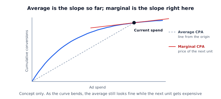
Average CPA asks: across everything spent so far, what did one conversion cost? A report card on the past.
Marginal CPA asks: if I spend one more unit right here, what will that unit's conversion cost? Scaling decisions need this one.
Ad channels generally follow diminishing returns. Cheap inventory and responsive audiences get consumed first, and larger budgets reach progressively more expensive people.
So this state is extremely common: average CPA sits under target while marginal CPA has already passed it. Scaling in that zone slowly degrades the average, and a few weeks later someone asks why CPA went up. That is exactly the cycle above.
Saturation is one ratio
No need to complicate it.
Saturation index = marginal CPA ÷ average CPA
- Near 1 — average and marginal efficiency are similar near the fitted point; larger scale changes are not guaranteed.
- Well above 1 — saturated. More spend buys proportionally less.
- Below 1 — headroom remains. Compare against target CPA, other channels’ marginal efficiency, observed ranges, and constraints before prioritizing.
Lower marginal ROAS relative to average ROAS signals saturation. The tool defines its ROAS saturation index as average ROAS ÷ marginal ROAS, keeping the same direction as the CPA index: higher means more saturated.
Campaign saturation analysis computes this index per channel from a CSV with date, channel, cost, and outcome.
Some channels will come back "withheld"
There is an important precondition here. A channel whose spend stayed flat cannot produce a curve.
Which makes sense — if every data point sits at the same spend level, the slope is unknowable. A channel that spent the same $50k every month contains no information at all about what $100k would do.
So some channels return a withheld verdict. That is not the tool failing; it is the data declining to answer. It is tempting to read that as an error and start changing options until a number appears, but a number produced that way is invented, not measured.
If more observations are needed, first define a spend-change plan with risk limits and comparison conditions. Duration depends on conversion delay, seasonality, and sample size. Two or three weeks of variation does not guarantee an identifiable curve or validity in the following quarter.
Saturated does not only mean "stop"
A saturation verdict is not an instruction to halt. Moving that budget to a channel with headroom can simulate improved efficiency without increasing total spend; actual improvement still needs validation.
Budget allocation simulator uses the per-channel curves to compute where to add and where to cut at the same total. The output is a scenario based on historical observations; it does not guarantee approval or improved efficiency.
If the question is where to move budget across several channels at once, marketing budget allocation is the next read; to rule out that the added spend merely displaced organic demand, see paid and organic cannibalisation.
Try this today
Take the channel that currently looks best and check how much its spend actually varied over the last 8–12 weeks. If it barely moved, that channel has no basis for a scaling decision right now — good CPA or not.
Before collecting more observations, specify a loss limit, comparison period, conversion maturity, and stopping rule. Before-and-after data alone does not identify a causal effect.
Limits of this approach
Saturation is an association-based estimate, not a causal experiment. It reads "when spend was this much, outcomes were that much" out of history and fits a curve to it.
So the curve moves when seasonality or competition moves. A curve fitted in summer does not describe November.
Before a large budget move, shift a small slice first and check whether reality follows the prediction — size the initial change using acceptable loss and the sample needed for validation rather than a fixed fraction.
If computing this per channel every cycle is tedious, upload your existing report CSV. Marginal CPA and saturation get calculated per channel, and channels without enough spend variation are honestly marked as withheld rather than given a fabricated number. Data is processed in your browser and never sent to a server.
A CPA under target is not automatically a scaling signal. Check what the last unit of spend costs first.